Surrogate Modeling for Pressure Drop using PartiNet

This notebook uses synthetic fluidized bed theory and trains machine learning models to predict pressure drop.

---

🧪 Objective

To build fast surrogate models that predict pressure drop in a gas-solid fluidized bed using Random Forest, Linear Regression, and MLP — trained on synthetic data derived from fluid mechanics theory.

---

⚙️ Libraries and Data Generation

import numpy as np
import pandas as pd
from sklearn.model_selection import train_test_split
from sklearn.preprocessing import StandardScaler
from sklearn.linear_model import LinearRegression
from sklearn.ensemble import RandomForestRegressor
from sklearn.neural_network import MLPRegressor
from sklearn.metrics import mean_squared_error, r2_score
import matplotlib.pyplot as plt
import seaborn as sns

# Generate synthetic dataset
np.random.seed(42)
n = 200
Ug = np.random.uniform(0.1, 2.0, n)
dp = np.random.uniform(50e-6, 500e-6, n)
rho_p = np.random.uniform(1000, 3000, n)
H = np.random.uniform(0.2, 1.0, n)
mu_g = 1.8e-5
rho_g = 1.2
g = 9.81

---

📘 Theory Recap

🔹 Archimedes Number

\[Ar = \frac{d_p^3 \rho_g (\rho_p - \rho_g) \cdot g}{\mu_g^2}\]

🔹 Minimum Fluidization Velocity $(U_{mf})$

\[Re_{mf} = \sqrt{33.72 + 0.0408 \cdot Ar} - 33.7\] \[U_{mf} = \frac{Re_{mf} \cdot \mu_g}{\rho_g \cdot d_p}\]

🔹 Pressure Drop $(\Delta P)$

\(\text{For } U_g > U_{mf}\):

\[\Delta P = (\rho_p - \rho_g) g H\]

\(\text{For } U_g \leq U_{mf}\):

\[\Delta P = (\rho_p - \rho_g) g H \left( \frac{U_g}{U_{mf}} \right)\]

🔹 Solid Holdup $(\varepsilon_s)$

\[\varepsilon_s = \text{clip} \left(0.6 - 0.25 \cdot \frac{U_g}{U_{mf} + 1e-5}, 0.1, 0.6 \right)\]

---

🧲 Dataset Construction

Ar = (dp**3 * rho_g * (rho_p - rho_g) * g) / (mu_g**2)
Re_mf = (33.7**2 + 0.0408 * Ar)**0.5 - 33.7
Umf = Re_mf * mu_g / (rho_g * dp)
dP = (rho_p - rho_g) * g * H * (Ug > Umf) + (rho_p - rho_g) * g * H * (Ug <= Umf) * (Ug / Umf)
eps_s = np.clip(0.6 - 0.25 * (Ug / (Umf + 1e-5)), 0.1, 0.6)

data = pd.DataFrame({
    'Ug': Ug,
    'dp': dp * 1e6,
    'rho_p': rho_p,
    'H': H,
    'Umf': Umf,
    'dP': dP,
    'eps_s': eps_s
})

---

🛠️ Model Training

features = ['Ug', 'dp', 'rho_p', 'H']
target = 'dP'
X = data[features]
y = data[target]

X_train, X_test, y_train, y_test = train_test_split(X, y, test_size=0.2, random_state=0)
scaler = StandardScaler()
X_train_scaled = scaler.fit_transform(X_train)
X_test_scaled = scaler.transform(X_test)

lr = LinearRegression().fit(X_train_scaled, y_train)
rf = RandomForestRegressor(n_estimators=100, random_state=0).fit(X_train_scaled, y_train)
mlp = MLPRegressor(hidden_layer_sizes=(64, 64), max_iter=20000, random_state=0).fit(X_train_scaled, y_train)

---

📊 Model Evaluation

y_pred_lr = lr.predict(X_test_scaled)
y_pred_rf = rf.predict(X_test_scaled)
y_pred_mlp = mlp.predict(X_test_scaled)

def print_metrics(name, y_true, y_pred):
    print(f"{name} R2: {r2_score(y_true, y_pred):.3f}, MSE: {mean_squared_error(y_true, y_pred):.2e}")

print_metrics("Linear", y_test, y_pred_lr)
print_metrics("Random Forest", y_test, y_pred_rf)
print_metrics("MLP", y_test, y_pred_mlp)

Linear R2: 0.949, MSE: 1.78e+06  
Random Forest R2: 0.990, MSE: 3.45e+05  
MLP R2: 1.000, MSE: 1.63e+04

---

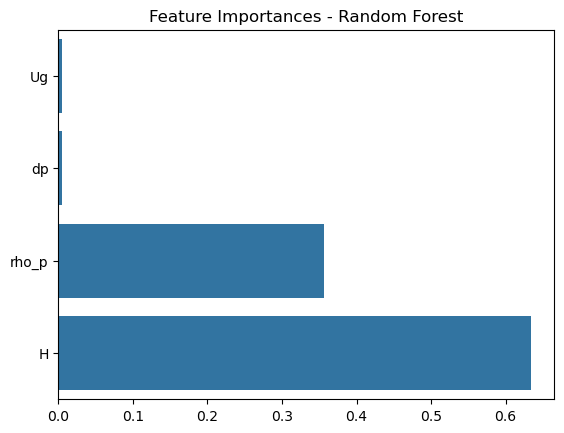
🔍 Feature Importance

importances = rf.feature_importances_
sns.barplot(x=importances, y=features)
plt.title("Feature Importances - Random Forest")
plt.show()

---

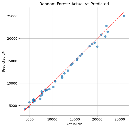
🎯 Predictions vs Actual

# Random Forest
plt.figure(figsize=(6, 6))
plt.scatter(y_test, y_pred_rf, alpha=0.7)
plt.plot([y_test.min(), y_test.max()], [y_test.min(), y_test.max()], '--r')
plt.xlabel("Actual dP")
plt.ylabel("Predicted dP")
plt.title("Random Forest: Actual vs Predicted")
plt.grid(True)
plt.show()

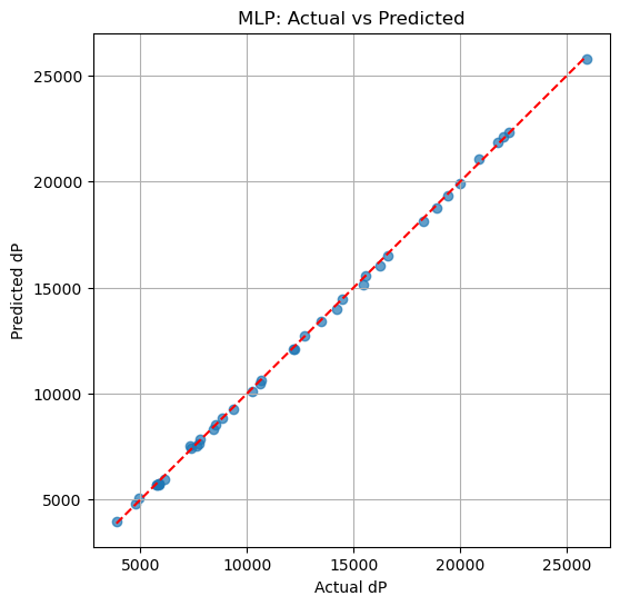
# MLP
plt.figure(figsize=(6, 6))
plt.scatter(y_test, y_pred_mlp, alpha=0.7)
plt.plot([y_test.min(), y_test.max()], [y_test.min(), y_test.max()], '--r')
plt.xlabel("Actual dP")
plt.ylabel("Predicted dP")
plt.title("MLP: Actual vs Predicted")
plt.grid(True)
plt.show()

---

🧫 Conclusion

PartiNet v1 achieves:

• 💡 Near-perfect fit using MLP (R² ≈ 1.00)
• ⚡ Real-time pressure drop predictions based on fluid bed physics
• 🚀 Ready for extension to 2D/3D CFD-DEM simulation data

---